For one of my research projects - in which I measure user satisfaction with the top-N recommendations presented to them - I report p-values of my employed statistical tests and the corresponding effect sizes 1. My advisor pushed me further to explain what it means given a value of an effect size. So here comes the post. In this post I only discuss Cohen’s effect size and Cliff delta effect size.
Cohen’s d
When we can assume that our data has a normal distribution and is on continous scale, then Cohen’s d effect size is an appropriate measure. So given a value of cohen’s d effect size (say 0.64), what does 0.64 mean?
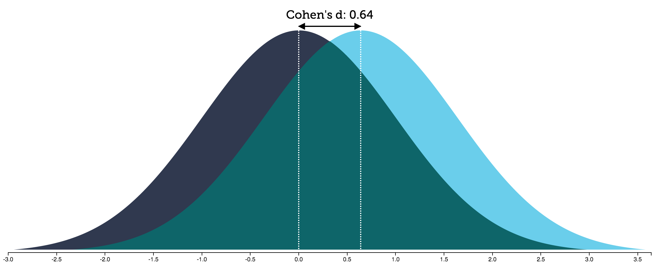
From the figure above, we can see that cohen’s d is just a distance of the two distributions’ means. However, it isn’t much helpful when saying that to our audience.
Fortunately, there are mathematical ways to interpret this distance, and I will describe my interpretation in a moment. Before reading my interpretation below, please imagine that we are measuring user satisfaction on a continuous scale, and that the two distributions above are the distributions of user satisfaction for two conditions. The distribution on the left is of the condition where users were presented bad top-N recommendations, and the distribution on the right is of the condition where users were presented good top-N recommendations.
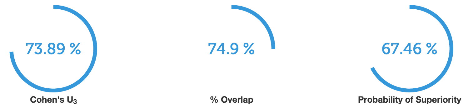
Thus, the cohen’s d of 0.64 tells me that about 74% of users presented with good top-N recommendations have the satisfaction levels that is above the average satisfaction level of users presented with bad recommendations. It also tells me that 75% of users in both conditions have the same levels of satisfaction. Moreover, when we pick two users at random - one of each condition - there is 67% chance we see that the user assigned with good recommendations is more satisfied that the one with bad recommendations.
Cliff’s delta
Unfortunately, in some cases our data isn’t that normal at all, and that the interested measure isn’t continuous. In particular, in my research the data is ordinal because users answered our survey on a 5-point scale. Thus Cliff’s delta comes to my rescue.
Cliff’s delta measure how often one value in one distribution is higher than the values in the second distribution. Translated this into the example above in which user satisfaction can be grouped into three levels: Satisfied, Neutral, Not Satisfied. Then we can measure how often users assigned with good recommendations were more satisfied than those with bad recommendations.
As demonstrated in the figure below, a cliff’s delta of 0.40 - with the corresponding cohen’s of 0.64 when the distritions are normal with continous scale - means that 53% of users assigned with good recommendations are more satisfied than those assigned with bad recommendations.
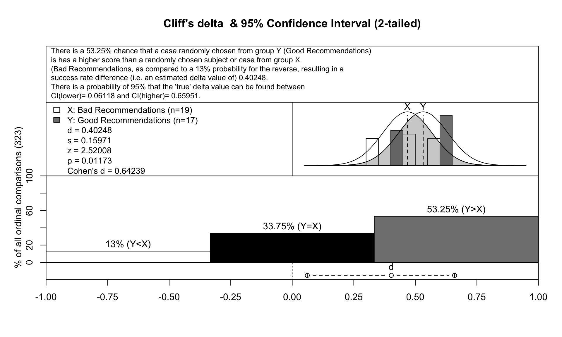
As we can see, with Cliff’s delta we cannot have as many information as we can with Cohen’s d. However, Cliff’s delta is a non-parametric approach thus we do not need to worry much about the distributions of our data.
Acknowledgement
I use the tool 2 to generate figures in Cohen’s d section and the ordom package in R to generate the figure in Cliff’s delta section.